Ridge EEG diagnostics for Amrith#
CURRENT FIGURES ARE SCHEMATIC
Amrith asked for visualization and analysis of the existing benchmark, not additional benchmarks. The immediate goal is to make the ridge baseline interpretable:
What EEG goes into ridge regression, what is predicted, and why can a simple linear model perform well?
Critical correction
The current repo baseline linear_ridge fits NumpyRidgeBaseline(alpha=1e-2) after reshaping [windows, time, channels] into [windows*time, channels]. It is therefore a regularized channel-to-channel linear map applied across stacked timepoints, not a giant flattened whole-window model.
What Amrith should see first#
The current EEG window and next-window target, with real channel labels and time units.
The design matrix actually passed to ridge: rows are
window x time, columns are channels/features.Actual vs predicted future EEG, plus residuals and per-channel metrics.
Autocorrelation and current-vs-next-window correlation, to test whether ridge is exploiting temporal continuity.
Ridge coefficient maps, to show whether the model mostly uses diagonal/same-channel structure or broad channel mixing.
Optional topomaps only if real montage/channel positions exist.
Current schematic figure packet#
These figures are layout prototypes generated by:
python3 scripts/analysis/plot_ridge_eeg_diagnostics.py
They are useful for visual grammar, but not evidence until rerun with real benchmark tensors.
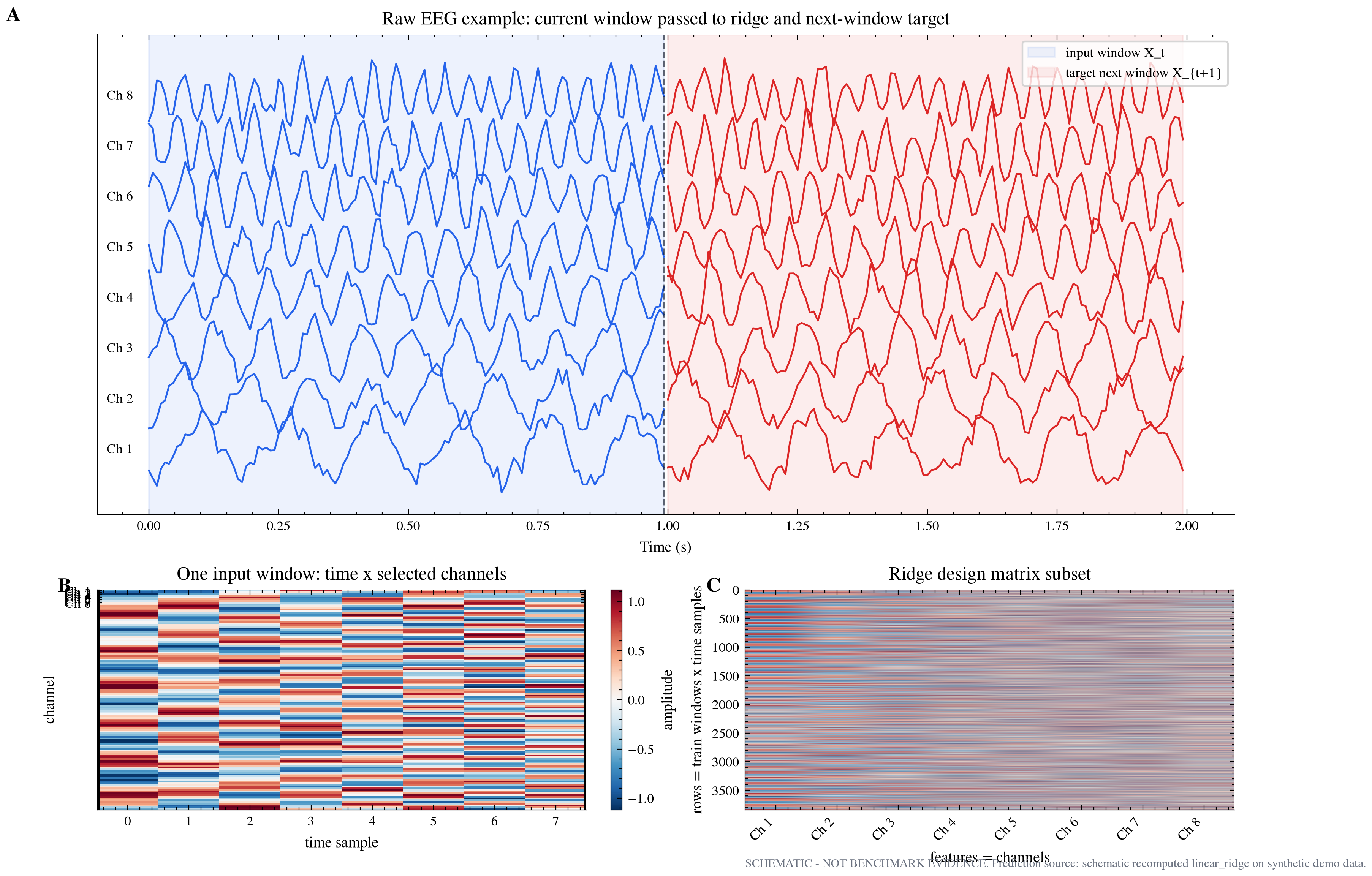
Figure 1. EEG input/target layout. Current window, next-window target, and the ridge design-matrix subset. In the real version, this must use actual channel names, sampling rate, split, and benchmark source.
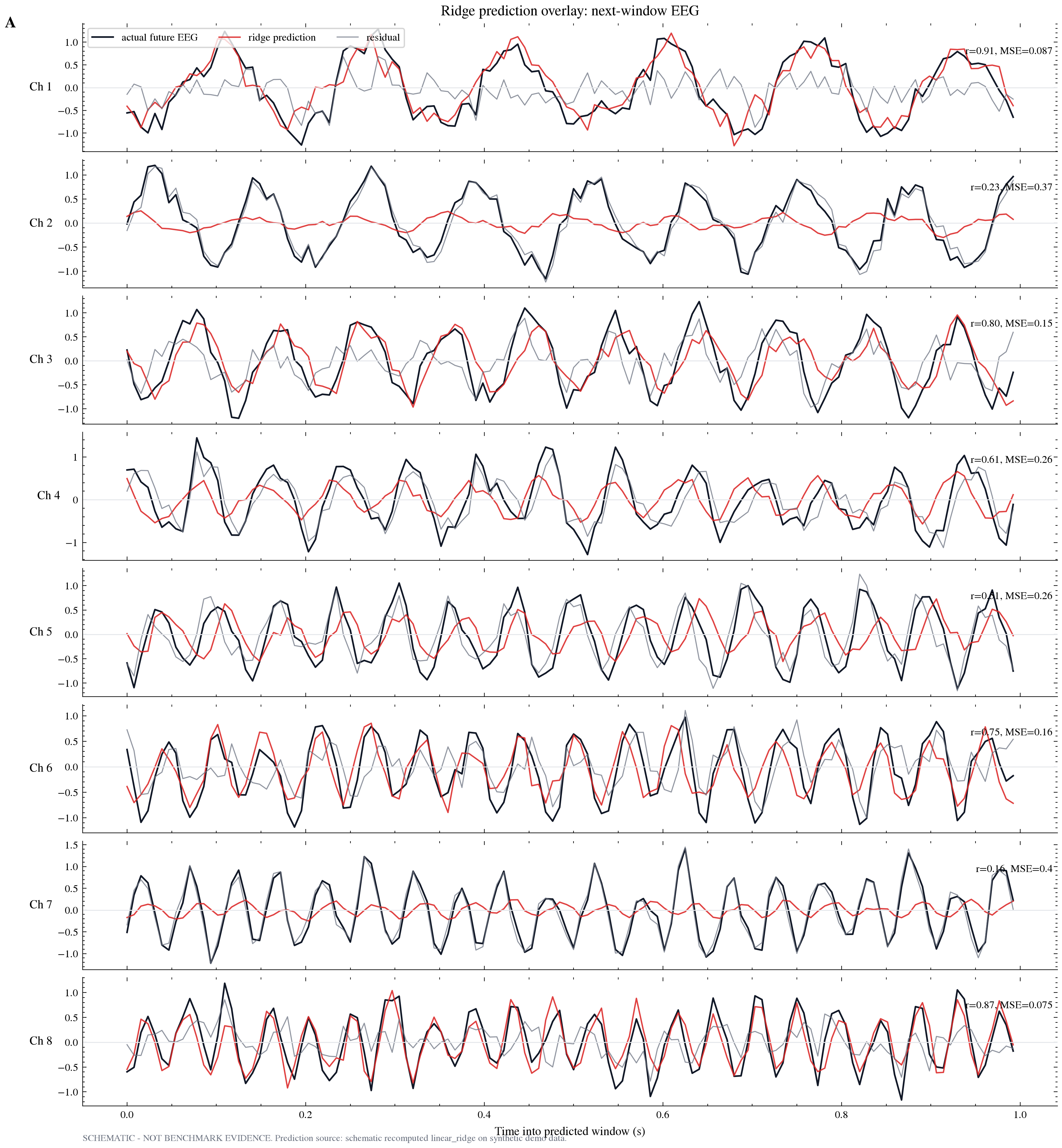
Figure 2. Prediction overlay. Actual future EEG, ridge prediction, and residuals. This is the main sanity-check figure for whether ridge tracks physiologically meaningful dynamics or mostly smooth continuity.
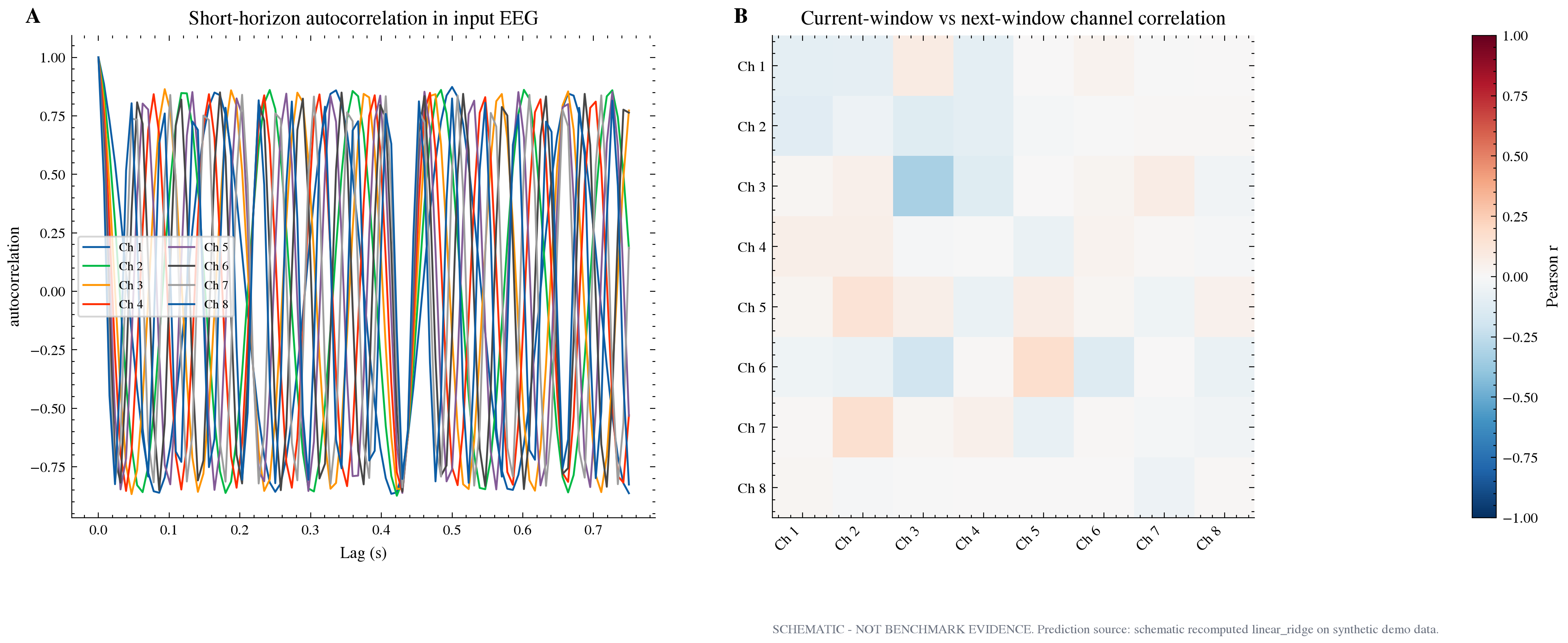
Figure 3. Autocorrelation and lag structure. If autocorrelation is strong over the forecast horizon, ridge can perform well without implying a rich neural-state model.
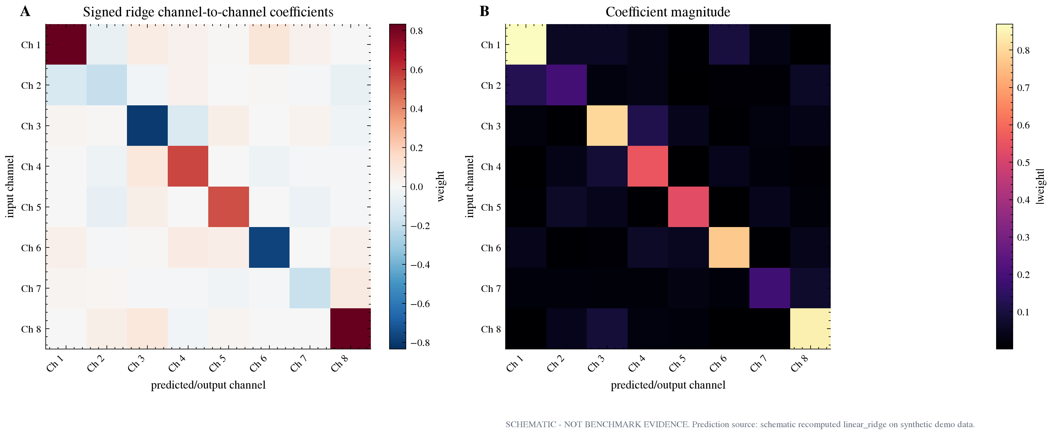
Figure 4. Ridge coefficient map. Shows signed and absolute channel-to-channel coefficients. A diagonal-heavy map would support a persistence/covariance explanation.
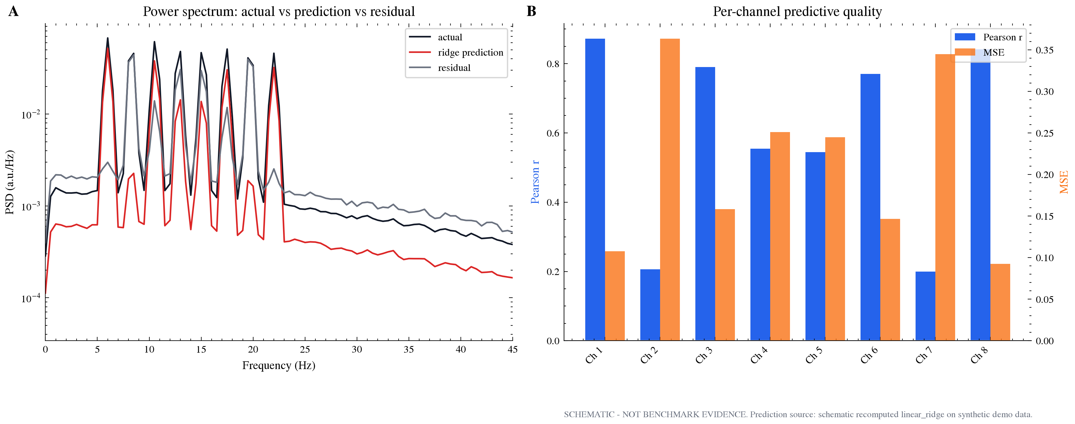
Figure 5. Spectral and residual diagnostics. Compares actual, predicted, and residual power spectra, plus per-channel prediction quality.
Real-data contract#
To convert these from schematic figures to benchmark-derived figures, create an .npz with:
x_train:[n_train_windows, time, channels]y_train:[n_train_windows, time, channels]x_test:[n_test_windows, time, channels]y_test:[n_test_windows, time, channels]optional
y_pred_test: benchmark/exported ridge predictionoptional
sfreq: sampling frequencyoptional
channel_names: EEG channel namesoptional provenance fields:
dataset,task_id,split_manifest,event_manifest,commit,run_label
Then run:
python3 scripts/analysis/plot_ridge_eeg_diagnostics.py \
  --npz path/to/ridge_eeg_tensors.npz
If the arrays are flattened, add:
  --time-length 128 \
  --n-channels <N>
Suggested mentor-facing interpretation#
A conservative caption should say:
The ridge baseline is analyzed as a regularized linear channel-to-channel map over stacked timepoints for the current EEG future-state task. These diagnostics test whether ridge performance reflects short-horizon temporal autocorrelation and stable channel covariance, rather than evidence of a complex latent neural field model.
That framing is careful, honest, and exactly the kind of thing a mentor can trust.